Machine learning is the scientific discipline concerned with the design and development of algorithms that allow computers to infer knowledge from input data. The knowledge inferred is the novel and potentially useful relationships between data elements. Within the scope of machine learning, supervised and unsupervised techniques can be distinguished.

Unspervised vs supervised learning

Unsupervised learning refers to the problem of trying to find hidden structures in a set of unlabelled data instances. That is, previously unlabelled data instances are labelled by finding groups of homogeneous instances within the data. Homogeneity is usually measured by some distance measure. For example, the $k$-means algorithm iteratively assigns instances to $k$ clusters within the feature space. The objective of the algorithm is to find a clustering in which the total distance between a cluster centroid and all the instances assigned to a cluster is minimized.

Conversely, supervised learning is the task of fitting a function to a set of labelled data instances. The class labels can be continuous or discrete values. A function that maps a data instances into a continuous real valued class variable is called a regression function, whereas a function that maps a data instance into a discrete valued class variable is called a classification function or a classifier.

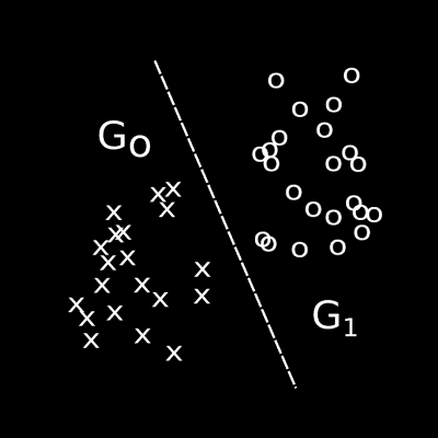
For example, given a set of labelled instances that belong to two groups, say, group A and group B. Supervised learning can be used to derive a classifier that will classify some previously unlabelled instance as belonging to either group A or group B.

Supervised learning

The goal of supervised learning is to derive a mapping from a set of input variables to an output variable using a set of example input-output variable pairs. The resulting mapping can then be used to infer an output variable value for instances where the input variables are known, but the value of the output variable is not known.

Formally, given a set of $N$ exemplar tuples $(\vec{x}^{(t)},y^{(t)})$, where each example $(t = 1, \dots, N)$ constitutes a predictor variable vector $\vec{x}^{(t)} = (\mathit{x_1,x_2,\dots,x_r})$ and an associated predicted variable $y^{(t)}$. In more complex problems there may be several predicted variables denoted by $y^{(t)}_l$ with $l=1, \dots, L$. The predicted variable is related to the predictor variables by some unknown function $y=f(\vec{x})$. Let the function $h(\vec{x})$ be a hypothesis of the true function $f(\vec{x})$ and let the loss function $L(y,h(\vec{x}))$ be some measure of the error between the actual dependent variable value $y=f(\vec{x})$ and the predicted dependent variable value $\hat{y}=h(\vec{x})$.

The objective of supervised learning is to find a function $h(\vec{x})$ that minimizes the generalization loss $R(h)$ over all possible tuples $(\vec{x},y)$ in population $\varepsilon$,

The probability distribution $p(\vec{x},y)$ for the population $\varepsilon$ is , however, not known. Therefore an estimate of the generalization loss, the empirical loss $R_{emp}(h)$, is calculated as the average loss over the exemplar tuple set,

An optimization algorithm searches through the space of all possible hypotheses $\mathbb{H}$ for the function $h^*$ that minimizes this empirical loss,

An exhaustive search of the hypothesis space quickly becomes computationally exhaustive, therefore, supervised learning involves heuristic approaches to search for a good enough function $h$ in $\mathbb{H}$. These approaches are called induction or learning algorithms.

Components of Supervised learning

Three primary components of a supervised learning technique can be identified: model representation, model evaluation and search method. Model representation involves choosing a family of models to be considered. The chosen model representation defines the hypothesis space $\mathbb{H}$. Model evaluation involves choosing a loss function with which to evaluate a candidate hypothesis $h$. Model search involves searching for the optimal hypothesis in the chosen hypothesis space $\mathbb{H}$.

The task of finding the best hypothesis $h \in \mathbb{H}$ can be further divided into two separate subtasks: model selection and parameter search. In model selection, also known as hyper-parameter search, different model specifications in the chosen family of model representations are considered. Given a fixed model specification, a parameter search is performed by some induction algorithm to find those parameters, which optimize the evaluation criteria over the example data set. Hyper-parameter search is implemented as an outer loop to the parameter search problem, within each loop the parameter search is focussed on a different region of the hypothesis space $\mathbb{H}$¹.

For example, consider fitting a function to a data set. First, select the type of function one wants to fit to the data, say a polynomial function. Secondly, select a loss function with which to measure all candidate polynomials considered, say the mean-squared-error loss function. Thirdly, find the polynomial function that minimizes the average mean-squared-error over the example data set. In looking for the optimal polynomial, consider polynomials of different degrees (hyper-parameter search), and consider polynomials with the same degree but different term coefficients (parameter search).

Learning or induction algorithm

Various polynomial regression techniques (induction algorithms) can be used to find the optimal term coefficients (parameter search) once the optimal degree has been chosen (hyper-parameter search).

As stated, the objective of supervised learning is to find a hypothesis function $h\in \mathbb{H}$ that closely approximates the true function $f$. Two types of problems can be addressed using supervised learning techniques: regression problems and classification problems. If the image of the true function $f$ is an infinite set of real values then the supervised learning problem is called a regression problem and the hypothesis function $h$ is called the regression function. Alternatively, if the image of the true function $f$ is a finite set of integers (or class labels) then the supervised learning problem is called a classification problem and the hypothesis function $h$ is called a classifier.

Several supervised learning techniques exist with which to derive a classification function from an exemplar data set, including decision trees, naive Bayes classifiers and Bayesian networks, neural networks, discriminant functions, $k$-nearest neighbour classifiers and support vector machines. After learning, each of these classifiers has the ability to return a class label $\hat{y}$, from a predefined set of class labels, when presented with an input pattern $\vec{x}$. There is, however, no golden rule with regard to the best supervised learning technique to use for a particular problem, as the performance of the various techniques is much influenced by the particular application domain.

Results from the StatLog project² show that the $k$-nearest neighbour classifier, the MLP neural network classifier and the linear discriminant classifier consistently perform relatively well in most application domains.

The classification problem

Many examples of classification problems can be listed in the field of marketing, telecommunication, healthcare, human resource management, finance and so forth. Examples include face detection, as well as facial recognition; speech recognition; bankruptcy and credit scoring; spam detection; document classification; financial crime detection , as well as churn detection.

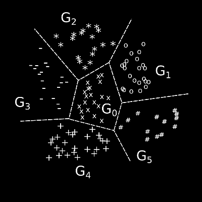
In each of these problem domains a function $h$ has to be found that accurately maps an observed object into a finite set of predefined class labels. In a $n$ class classification problem the function $h$ has to map an observed object into one of $n$ possible class labels. In a binary classification problem the function $h$ has to map an observed object into one of two possible class labels.

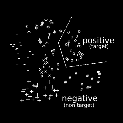
Multiple class classification is essentially more challenging than a binary class classification problem, since the induced classifier must learn how to distinguish between a larger number of classes simultaneously. Therefore, it is often required to transform a multiple class classification problem into a set of binary classification problems because many supervised learning techniques have a disadvantage in efficiently separating multiple classes. A multiple class problem can be decomposed into a set of binary subproblems by either comparing one class against all other classes or by comparing one class against another class. In a one-against-all decomposition each class is opposed to all the others classes, thus giving $n$ subproblems. In a one-against-one decomposition each class is opposed to each other class, thus giving $n(n-1)/2$ subproblems. possible combination of classes.

For example, in a $6$-class classification problem a multiple class classifier $h$ will classify an instance into any one of the possible classes, with $h \rightarrow \{G_0,...,G_5\}$. A one-against-all binary classifier $h$ will confirm or refute that an instance belongs to the modelled target class, for example $h \rightarrow \{G_1 (\text{positive}), \text{\ not\ } G_1 (\text{negative})\}$. A set of $6$ classifiers can be constructed by using each class in turn as the target. A one-against-one binary classifier $h$ will assign instances into one of two classes, for example $h \rightarrow \{G_0,G_1\}$. A set of $15$ classifiers can be constructed, one classifier for each. See figure below.

When transforming a multiple class problem into a set of binary subproblems a method is needed with which to combine the solutions of the binary subproblems into a solution for the multiple class problem. When using the one-against-all method the class with the highest output probability is usually chosen. In the one against-all strategy, the majority vote over the individual classifier outputs are taken - a technique called round robin binarization. The best scheme to use varies according to the application domain and the supervised learning technique used.

Notes

• Originally published as part of Wilgenbus, E.F., 2013. The file fragment classification problem: a combined neural network and linearprogramming discriminant model approach. Masters thesis, North West University.

References

Related tags

emerging technologydata and decision sciencemachine learning