Neural networks imitate the cognitive function of the brain to approximate intelligent machines [^n002]. The neuron, shown in the Figure below, is the fundamental building block of the human brain. The neuron is a special type of cell that processes and transmits information electrochemically. Individually each neuron receives nerve impulses from preceding connected neurons through connections called dendrites. Each input received is amplified or reduced according to the receiving neuron's learned sensitivity to inputs originating from each connected sender neuron. Within the cell body, the adjusted input signals are aggregated and an output signal is calculated. The output signal is transmitted on the axon. The axon in turn is the connection point for multiple successive neurons.

A biological neuron

The ability of the human brain to encode knowledge is realized by signals sent within a complex network of roughly 100 billion neurons, each neuron connected to several thousand other neurons [^book_olson]. Each neuron's ability to alter its sensitivity to the various inputs it receives contributes a tiny bit to the overall network's computational capacity.

Artificial neural networks originated from attempts to mimic the learning ability of the human brain [^nn001]. In this section artificial neural networks are introduced. The first subsection outlines the perceptron and the multilayer perceptron neural network model. The second subsection introduces the back propagation algorithm, a parameter optimization method used to induce neural network classifiers. The third subsection introduces the concept of over fitting, as well as techniques that can be used to prevent over fitting. The last subsection lists advantages and disadvantages of MLP neural network classifiers.

Perceptrons and multilayer perceptrons

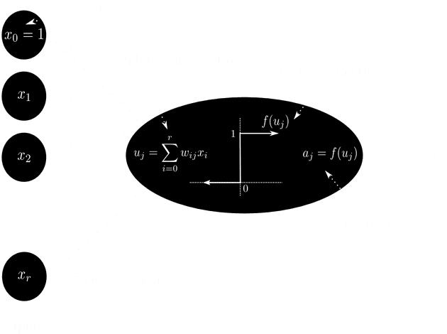
In the same manner as the human brain, an artificial neural network is composed of nodes connected by directed network links [^book_russels]. The net-input $u_j$ to some node $j$ is computed by combining the input signals $x_1$ to $x_r$ in a weighted sum and adding a node bias $-\theta_j$. This is,

where the connection weight from input node $i$ to node $j$ is $w_{ij}$ and the bias is $\theta_j$. By introducing an extra dummy input signal $x_{0j}$ equal to one, the combination function can be written as [^book_bishop]

with $w_{0j}=-\theta_j$.

The node output $a_j$ is $1$ if the net-input $u_j$ is greater than or equal to $0$, else the node output is $0$. This hard limit function, or step function, can be written as

Such a node, called a perceptron, is depicted in Figure below.

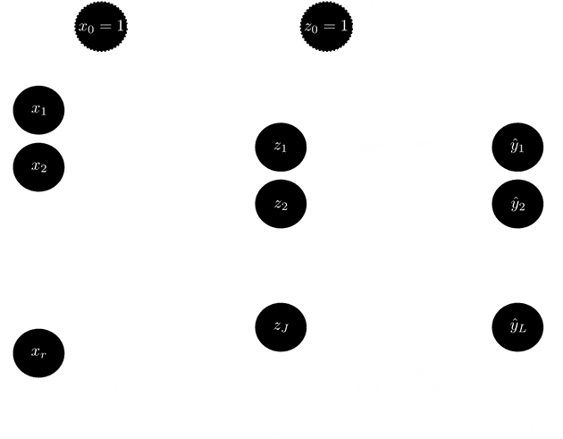
A feed-forward neural network is composed of multiple perceptrons interconnected in such a way as to allow the output of one perceptron to be the input to another perceptron [^book_bishop]. The connections in a feed-forward network only allow signals to pass in one direction. Specifically, the multilayer perceptron (MLP) neural network is the most widely studied and used feed-forward neural network model [^nn001]. Such a neural network is structured as three or more distinct layers: an input layer, one or more hidden layers, and an output layer. Each layer constitutes a set of nodes, with nodes from different layers being highly interconnected in a feed-forward manner: All nodes from the input layer are connected to all nodes in the first hidden layer, all nodes in the first hidden layer are connected to all nodes in the second hidden layer, and so forth, until all nodes in the last hidden layer are connected to all nodes in the output layer. The neural network maintains a vector of connection weights used to adjust the input signal as it propagates through the network towards the output layer. The structure of a three-layer MLP neural network is shown in the figure below.

This MLP neural network receives $r+1$ input signals at the input layer nodes. The input vector $\vec{x} \in R^{r+1}$ represents the $r$ input features $x_1$ to $x_r$ and the bias signal $x_0$ set equal to one. The input signal is propagated forward to $J$ hidden layer nodes. Each hidden layer node functions like a perceptron. The node input is computed as the weighted sum of inputs received from all preceding nodes. That is $u_j = \sum_{i=0}^{r}w_{ij}x_i$ where $w_{ij}$ is the weight of the connection between input node $x_i$ and hidden node $z_j$.

The hidden layer's output is computed by passing the weighted sum of inputs $u_j$ through an activation function $f^h(u_j)$. This activation function can be any monotonically increasing function, such as the symmetric sigmoid function [^book_steeb],

The output of the hidden layer is a vector $\vec{z} \in R^{J+1}$ with the bias signal $z_0$ set to one. The vector $\vec{z}$ supplies inputs to the output layer with $L$ nodes.

Similar to the nodes in the hidden layer, each output layer node functions like a perceptron. Input signals from the hidden layer nodes are combined in a weighted sum $u_l = \sum_{j=0}^{J}w_{jl} z_j$ where $w_{jl}$ is the weight of the connection from hidden node $z_j$ to output layer node $\hat{y}_l$. The output layer produces a vector $\hat{\vec{y}} \in R^{L}$. Each output node produces output $\hat{y}_l$ by passing the weighted sum of inputs $u_l$ through a monotonically increasing activation function $f^o(u_l)$. For example, a logistic activation function can be used,

The entire MLP model can be represented as the following non-linear function,

for output $l=1 \dots L$, where $f^h$ and $f^0$ are the activation functions in the output layer and hidden layer respectively, and $\vec{w}\in R^{J(r+1)+L(J+1)}$ is the vector of connection weights [^book_russels].

Each connection weight $w \in \vec{w}$ is used to adjust the input signal as it propagates through the network towards the output layer. By maintaining a weight for each connection in the network, a signal originating from a node can be very important in generating the output of one node and unimportant in generating the output of another node. It is through this process of connection specific signal weighting that a neural network has its predictive power. It has been shown that a three-layer MLP neural network with enough hidden layer nodes can approximate any continuous function with any desired degree of accuracy [^hornik].

The process in which the optimal weights vector ${\vec{w}}^*$ is determined, hence the way the network ``learns", is commonly referred to as network training. The back propagation algorithm is a popular technique used for network training. Gaining a general understanding of this algorithm is important due to its significance in neural network literature and because it is used in the empirical study of this dissertation. The back propagation algorithm is outlined in the next subsection.

[^n002]: coming soon [^book_olson]: coming soon [^hornik]: coming soon [^nn001]: coming soon [^book_russels]: coming soon [^book_bishop]: coming soon [^book_bishop]: coming soon [^nn001]: coming soon [^book_steeb]: coming soon [^hornik]: coming soon */}